Fasten a spatial index to the unsuspecting OpenSource DBMS

I always liked it when the title clearly says what will happen next, for example, "Texas chainsaw massacre". So under the cut we add spatial search to the DBMS in which it initially had.

introductory
Let's dispense with General words about the importance and usefulness of spatial search.
To the question, why not take the open DBMS with embedded spatial search, the answer is this: "I want to get something done right, do it yourself"(With). But seriously, we will try to show that the most practical spatial problems can be solved in quite an ordinary desktop without the stress and extra costs.

As an experimental DBMS will use the open edition of the OpenLink Virtuoso. In its paid version available spatial indexing, but that's another story. Why this database? The author likes her. Fast, easy, powerful. Copied-launched-all works. Will only use regular tools With no plug-ins or special assemblies, only official build and a text editor.

index Type
We index the points using pixel-code (block) index.
What kind of pixel-code an index? This is a compromise swept curve, allowing to work with non-point objects in 2-dimensional search space. Combine to this class all the methods:
the

the
• in Some way divide the search space into blocks
the
• All blocks are numbered
the
• Each indexed object is assigned one or more numbers of blocks in which it is located
the
• in the search extent is split into blocks and for each unit or the continuous chain of units of a normal integer index (B-tree) get all the objects that belong to them.

The most known methods are:
the

the
• good Old Igloo (or other swept curve) with limited precision. Space cut the bars, the step which (usually) is the typical size of the indexed object. The cells are numbered as X...xY...yZ...z... ie by gluing the cell numbers of the normals.
the
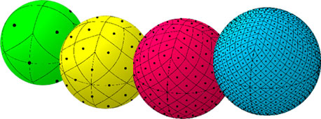
• HEALPix. The name comes from the Hierarchical Equal Area iso-Latitude Pixelisation. This method is designed to split the spherical surface in order to avoid the main disadvantage of Igloo different areas under cells at different latitude. The sphere is divided into 12 equal square sections, each of which is further hierarchically divided into 4 sub — plot. An illustration of this method is now in the header of the article
the
• Hierarchical Triangular Mesh (. HTM).This scheme of successive approximation to a sphere using triangles, since 8 start, each of which is hierarchically divided into 4 sub — triangle

One of the most famous circuits of block indices that is GRID. Spatial data are considered as a special case of the multidimensional index. At the same time:


the
1. space is cut in pieces using grid
the
2. the resulting cells are numbered in some way
the
3. data entered in a particular cell are stored together
the
4. attribute values are translated into numbers of cells along the axes using the “directory”, it is assumed that it is small and is placed in memory

if “directory” is large, it is split into levels a la the tree the

5. when you change, the grid can adapt, cells or columns to split, or, conversely, to merge
3-level GRID based on Z-order is used by DB2, 4-level GRID-based variant of the Hilbert curve used in MS SQLServer 2008

With all the disadvantages, the main of which, perhaps, is needapresent, need to adjust the index for a specific task, the block indexes there are pluses: simplicity and pantophagy. In essence it is an ordinary tree with additional semantic load. We somehow convert the geometry to numbers in the index and in the same way we get the keys to search the index.

data Type
Why? As already mentioned, the Block indexes, all the same what to index. The rasterizer for points trivial, but for polygons it would have to write, and it is completely irrelevant to the topic.

data Itself
Without further ADO,
the

put point on the lattice sites 4000Х4000 with the origin at (0,0) and step 1. the

• will receive a square of 16 million points.

the cell block index will take for 10X10 the

• so we have a 400X400 cells each with 100 points.

For an index, no matter how points are located inside the cell, and we kind of regularity will allow you to control the correctness of the results.

To generate the data we use here such script AWK(though, to be 'data'.awk'):
the

BEGIN {
cnt = 1; sz = 4000;
# Set the checkpoint interval to 100 hours -- enough to complete most of the experiments.
print"checkpoint_interval (6000);"; 
print"SET AUTOCOMMIT MANUAL;";
for (i=0; i < sz; i++) {
for (j=0; j < sz; j++) {
print "insert into \"xxx\".\"YYY\".\"_POINTS\"";
print " (\"oid_\",\"x_\", \"y_\") values ("cnt","i","j");";
cnt++;
}
print"commit work;"
}
print"checkpoint;"
print"checkpoint_interval (60);"; 
exit;
}

Server
the

the
• Use the official Bild from the company website.
  The author used the latest version 7.0.0 (x86_64), but it does not matter, you can take any other.
the
• is Installed, if not, Microsoft Visual C++ 2010 Redistributable Package (x64)
the
• Choose the directory for tests and copy there libeay32.dll, ssleay32.dll, isql.exe, virtuoso-t.exe from the archive 'bin' and virtuoso.ini from the archive 'database '
the
• start the server using 'start virtuoso-t.exe +foreground', allow the firewall to open ports
the
• Test the availability of the server with the command 'isql localhost:1111 dba dba'. After the connection is established, enter, for example. 'select 1;' and make sure that the server is alive.

Datasheet
To begin, create a table of points, nothing more:
the

create user "YYY";
create table "xxx"."YYY"."_POINTS" (
"oid_" integer,
"x_" double precision,
"y_" double precision,
primary key ("oid_") 
);

Now the actual code:
the

create table "xxx"."YYY"."_POINTS_spx" (
"node_" integer, 
"oid_" integer references "xxx"."YYY"."_POINTS", 
primary key ("node_", "oid_") 
);

where node_ is the ID of the cell space. Note that, although the index is created as a table, both fields are primary keys and hence, Packed into the tree.

Custom index options:
the

registry_set ('__spx_startx', '0');
registry_set ('__spx_starty', '0');
registry_set ('__spx_nx', '4000');
registry_set ('__spx_ny', '4000');
registry_set ('__spx_stepx', '10');
registry_set ('__spx_stepy', '10');

System function registry_set allows you to record string pairs name/value to the registry is much faster than keeping them in an auxiliary table and still covered by the transactions.

Trigger on entry:

create trigger "xxx_YYY__POINTS_insert_trigger" after insert 
on "xxx"."YYY"."_POINTS" 
referencing new as n
{
declare nx, ny integer;
nx := atoi (registry_get ('__spx_nx'));
declare startx, starty double precision;
startx := atof (registry_get ('__spx_startx'));
starty := atof (registry_get ('__spx_starty'));
declare stepx, stepy double precision;
stepx := atof (registry_get ('__spx_stepx'));
stepy := atof (registry_get ('__spx_stepy'));
declare sx, sy integer;
sx := floor ((n.x_ - startx)/stepx);
sy := floor ((n.y_ - starty)/stepy);
declare ixf integer;
ixf := (nx / stepx) * sy + sx;
insert into "xxx"."YYY"."_POINTS_spx" ("oid_","node_") 
values (n.oid_,ixf);
};

Put all of this in, for example, 'sch.sql' and execute by

isql.exe localhost:1111 dba dba <sch.sql

Download data
Once the schema is ready, you can fill in data.
the

gawk -f data.awk | isql.exe localhost:1111 dba dba >log 2>errlog

it took the author of 45 minutes (~6000 per second) on Intel i7-3612QM 2.1 GHz 8Gb memory c.
The memory size occupied by this server was 1 Gb, the database size on disk — 540Mb, i.e. ~34 bytes for its index.
Now you should verify that the result is correct, you enter in isql
the

select count(*) from "xxx"."YYY"."_POINTS";
select count(*) from "xxx"."YYY"."_POINTS_spx";

Both queries should produce 16 000 000.

As a guide you can use the data published by the here:
.
They obtained for PostgreSQL(Linux), 2.2 GHz Xeon.
On the one hand, the data obtained 9 years ago. On the other, in this case, the bottleneck are disk operations, random access to the disk in the intervening period has accelerated not so much.
It should be noted that the shading data and then indexing occurs (for obvious reasons) is significantly faster than indexing on the fly. But we are more interested in indexing it on the fly because for practical purposes more interesting spatial DBMS, not spatial search system.

And yet, it should be noted that when pouring the spatial data is very important the order in which they fill.
In this paper and in the above mentioned order of presentation of points was a perfect (or close to it) from the point of view of the spatial index. If the data mix, the performance drops quite dramatically regardless of the chosen DBMS.
If the data arrives randomly, we can recommend storing them in the sump, the overflow sort and pour portions.

Establish search
We will use such a great feature of the Virtuoso, as a procedural view.
the

create procedure "xxx"."YYY"."_POINTS_spx_enum_items_in_box" (
in minx double precision, 
in miny double precision, 
in maxx double precision, 
in maxy double precision)
{
declare nx, ny integer;
nx := atoi (registry_get ('__spx_nx'));
ny := atoi (registry_get ('__spx_ny'));

declare startx, starty double precision;
startx := atof (registry_get ('__spx_startx'));
starty := atof (registry_get ('__spx_starty'));

declare stepx, stepy double precision;
stepx := atof (registry_get ('__spx_stepx'));
stepy := atof (registry_get ('__spx_stepy'));

declare sx, sy, fx, fy integer;
sx := floor ((minx - startx)/stepx);
fx := floor (1 + (maxx - startx - 1)/stepx);
sy := floor ((miny - starty)/stepy);
fy := floor (1 + (maxy - starty - 1)/stepy);

declare mulx, muly integer;
mulx := nx / stepx;
muly := ny / stepy;

declare res any;
res := dict_new ();
declare cnt integer;
for (integer declare iy, iy := sy; iy < fy; iy := iy + 1) 
{
declare ixf, ixt integer;
ixf := mulx * iy + sx;
ixt := mulx * iy + fx;
for select "node_", "oid_" from "xxx"."YYY"."_POINTS_spx" 
where "node_" >= ixf and "node_" < ixt do 
{
dict_put (res, "oid_", 0);
cnt := cnt + 1;
}
}
declare arr any;
arr := dict_list_keys (res, 1);
gvector_digit_sort (arr, 1, 0, 1);

result_names(sx);
foreach (integer oid in arr) do 
{
result (oid);
}
};
create procedure view "xxx"."YYY"."v_POINTS_spx_enum_items_in_box" as
"xxx"."YYY"."_POINTS_spx_enum_items_in_box" (minx, miny, maxx, maxy) ("oid" integer); 

In essence, this procedure is very simple, she finds out which cell block index falls search extent, and for every line of those cells is doing under request records the IDs of entries in the hash map, while eliminating duplicates and gives the resulting set of IDs as the result.
How to use the spatial index? For example:
the

select count(*), avg(x.x_), avg(x.y_) from
"xxx"."YYY"."_POINTS" as x, xxx."YYY"."v_POINTS_spx_enum_items_in_box" as a
where a.minx = 91. and a.miny = 228. and a.maxx = 139. and a.maxy = 295. 
and x."oid_" = a.oid 
and x.x_ > = 91. and x.x_ < 139. and x.y_ > = 228. and x.y_ < 295.;

Here is the join between the points table and synthetic recordsets of the procedural view by ID. Here procedural view plays the role of the rough filter, which works exactly the cell. Therefore, in the last line we placed a thin filter.
Expected result:
the

the
• Number: (139 — 91) * (295 — 228) = 3216
the
• Average X: (139 + 91 — 1) / 2 = 114.5 (-1 because right border excluded)
the
• Secondary Y: (295 + 228 — 1) / 2 = 261 (...)

so here is one query in one transaction we performed a spatial search.

Benchmark
For making the flow of queries, I use the following AWK script:
the

BEGIN {
srand();
for (i=0; i < 100; i++) {
for (j=0; j < 100; j++) {
startx = int(rand() * 3900);
finx = int(startx + rand() * 100);
starty = int(rand() * 3900);
finy = int(starty + rand() * 100);
print "select count(*), avg(x.x_), avg(x.y_) from";
print "\"xxx\".\"YYY\".\"_POINTS\" as x, "
print "\"xxx\".\"YYY\".\"v_POINTS_spx_enum_items_in_box\" as a"
print "where a.minx = "startx". and a.miny = "starty"."
print " and a.maxx = "finx". and a.maxy = "finy". and"
print "x.\"oid_\" = a.oid and x.x_ >= "startx". and x.x_ < "finx"."
print " and x.y_ >= "starty". and x.y_ < "finy".;"
}
}
exit;
}

As you can see, it turns out 10,000 queries in random places with random size (0...100). Prepare 4 set and perform three series of tests — one run isql with the tests, 2 parallel and 4 parallel. On an eight-core processor, more parallelization does not make sense. Let's measure the performance.
the

the
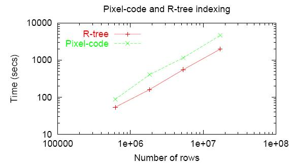
• stream 1: 151 sec = ~66 requests per second per thread
the
• 2 flow: 159 sec = ~63...
the
• 4 threads: 182 sec = ~55...

You can try to compare these times with the add obtained by spinal by means of two conventional indices for x_& & y_. We will index the table by those fields and run a similar series of tests with queries like
"xxx"."YYY"."_POINTS" as x where x.x_ > = 91. and x.x_ < 139. and x.y_ > = 228. and x.y_ < 295.; the Result is: a series of 10,000 queries is performed for 417 seconds with 24 queries per second.

Opinion
The presented method has several disadvantages, chief among which, as already noted, is the need to configure it for a specific task. Its performance is heavily dependent on settings that can not be changed after creating the index. However, this is true for most spatial indexes at all.

But even this written on the knee index gives a tolerable performance. Furthermore, since we control the whole process, on this basis it is possible to do whiter complex structures, for example, many table indexes to build that the regular methods is difficult. But about it somehow next time.

Article based on information from habrahabr.ru